on
Tensors Demystified
Tensors are rather infamously introduced in physics classes with the following tautology:
a tensor is an object that transforms like a tensor.
When I was first trying to learn general relativity, I was frustrated by the lack of intuition I had when working with tensors. The vast majority of resources on this topic are either far too theoretical for beginners or lack motivation for why tensors are physical. My goal with this post is to make tensors appear as natural and motivated generalizations of vector spaces and explain why they are ubiquitous in our best theories of physics.
⁂
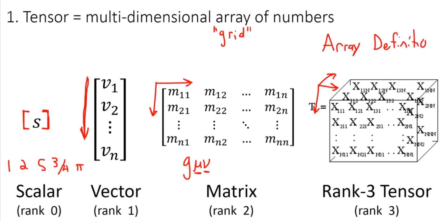
In computer science, a “tensor” of rank \(n\) refers to a multi-dimensional array where \(n\) indices are required to index any element. In physics and mathematics, this is not enough. We demand more: our tensors must transform in a certain manner under a change of coordinates in order to ensure they faithfully represent something geometric.
To see this, let’s step back and talk about what constitutes a vector, which is a rank \(1\) tensor. Not every list of numbers can be a vector: if I take the number of apples, grapes, and lemons I bought at the grocery store, this fails to form a vector because it does represent any underlying geometric object. On the other hand, displacement is a vector (e.g. the vector extending between my chimney and my fireplace). If I choose different basis vectors, or rotate my coordinate system, the coordinates I use to represent the displacement may change, but the underlyling geometric object remains unchanged (which I whimsically think of as a giant imaginary arrow). In contrast, position, which extends from the origin of our coordinate system to a given point in space, is not a vector. If we change the origin of our coordinate system, the underlying object does actually change, and hence the coordinates do not transform like a vector.
We can formalize this as follows for a point \(x \in \mathbb{R} ^n\)
\(\displaystyle x_{j'} = \sum^n_{i=0} R_{ij} x_i\),
where \(R\) is the rotation matrix.
I personally prefer to put the primes on the indices as opposed to the letter to emphasize that the underlying object is unchanged, but the alternative convention is often employed in the literature.
In this article, we will be using Einstein notation, where we drop the sigma notation and implicitly assume summation over repeated indices in the same term. Under this scheme, matrix multiplication is defined as follows:
\(\displaystyle C = A B \implies C_{ik} = A_{ij} B_{jk}\).
where an implicit summation is occurinng over the \(j\) index from \(1\) to \(n\). In the equations above, I have chosen to make all indices lower indices, although for technical reasons that I will explain later, this is not completely correct. We will soon transition to using superscripts; please assume that all superscripts are upper indices rather than exponents.
⁂
Every vector space has an associated dual space \(V^*\), which is defined as the vector space formed by all linear maps from \(V^* \rightarrow \mathbb{R}\). That is say, a function \(\omega : V \rightarrow \mathbb{R}\) is a covector (also called a dual vector, one-form, or linear functional) if and only if:
\(\displaystyle \omega(a \vec{u} + b{\vec{v}}) = a \omega(\vec{u}) + b \omega(\vec{v})\).
In a finite dimensional space, covectors are referred to as row vectors, since linear transformations to a scalar in finite dimensional space correspond to \(1 \times n\) matrices. We can introduce a dual basis \(\{\epsilon^1, \epsilon^2 ,\epsilon^3...\}\) defined as follows:
\(\displaystyle \epsilon^i(e_j) = \delta_{ij} = \begin{cases} 1 & \text{if } i = j,\\[4pt] 0 & \text{if } i \neq j. \end{cases}\).
where \(\delta_{ij}\) is the Kroenecker delta.
Observe that in the finite-dimensional case, every covector \(\omega \in V^*\) takes the form \(\omega(\vec{v}) = \vec{u} \cdot \vec{v}\), meaning \(V \cong V^*\) (where here \(\cong\) denotes isomorphism). We can convert any vector \(v \in V\) into its dual \(\omega \in V^*\) and vice versa in this manner. You could also arrive at the fact that \(V \cong V^*\) by recalling that all finite dimensional vector spaces of the same dimension are isomorphic. Quite interestingly, this isomorphism does not hold up in infinite dimensions, where \(V^*\) is in some sense “bigger” than \(V\), except under special conditions.
It is useful to think of covectors and vectors as “annihilating” each other. One can also regard basis vectors as linear functions from \(V^* \rightarrow \mathbb{R}\). It is convention to identify elements of \(V\) with their counterparts in \(V^{**}\) (that is, the dual of the dual). This allows us to say things like:
\(\displaystyle e_i(\epsilon^j) = \delta_{ij}\).
In two dimensions, we can visualize covectors as a stack of equally spaced lines, with each line associated with an integer (see figure 2). Observe that a vector whose endpoint falls on a labeled line evaluates to the associated integer, allowing us to think of the covector as a function that counts how many stacks have been “pierced” by the vector. More generally, \(n\)-dimensional covectors can be represented by a stack of equally spaced parallel \(n-1\) dimensional hyperplanes.
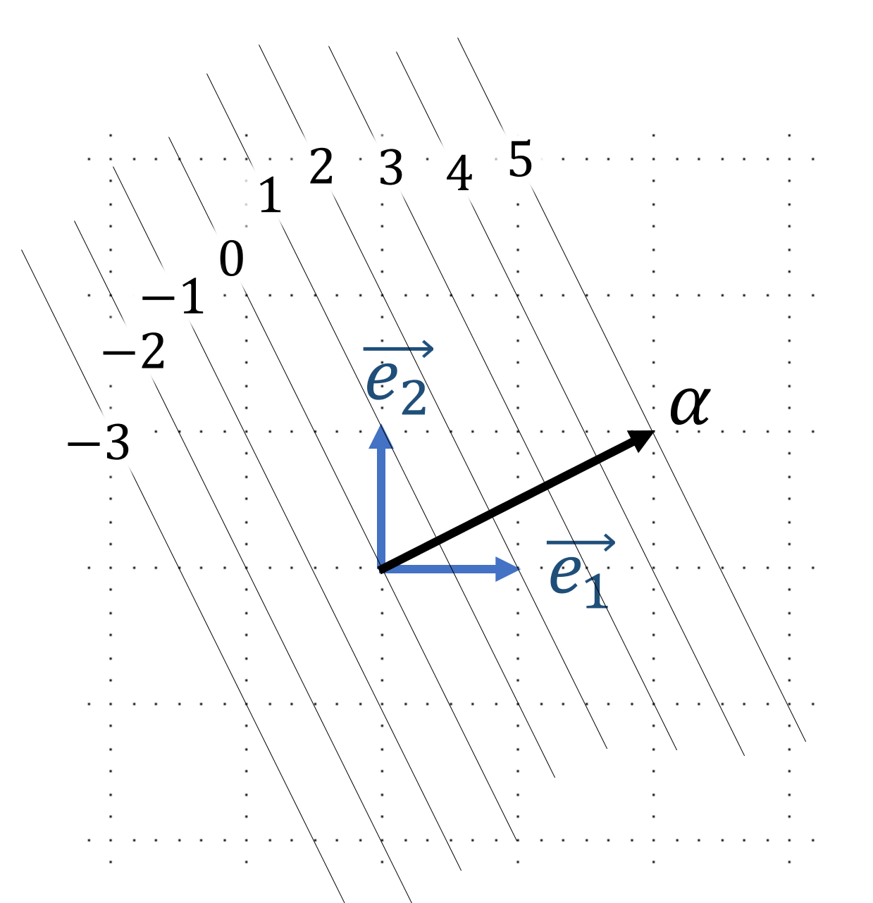
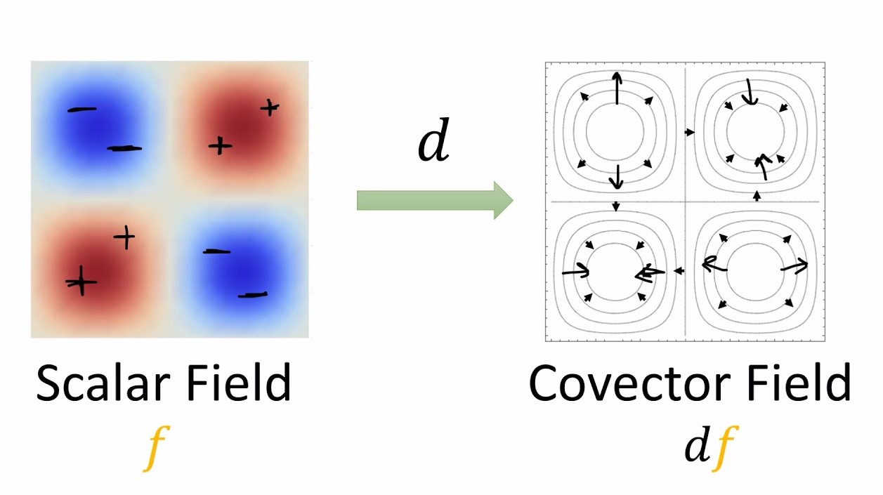
Observe that \(2 \omega\) has a covector stack that is twice as dense as \(\omega\) and \(\omega/2\) has a covector stack that is half as dense. One can imagine a sufficiently smooth covector field as a series of directed countour lines, which upon “zooming in” appear locally like a bunch of stacked lines. A good example of a covector field are fields of differential forms. Let \(f\) be a scalar field on \(\mathbb{R}^n\). The exterior derivative \(d\) is defined as the \(df(\vec{v}) = \nabla f \cdot \vec{v}\) (that is to say \(df\) is dual to \(\nabla f\)). One can visualize this process as taking in our scalar field and generating the covector field associated with its directed level sets (see figure 3).
Another useful intuition I like to use is to think of the scalar field as voltage and the resulting covector field as the dual of the electric field. In this analogy, the covector field can be thought of as consisting of equipotential surfaces, one of which is ground.
⁂
I now present to you the definition of a tensor:
A tensor \(T\) of rank \((k,l)\) is a multilinear map from a collection of dual vectors and vectors to \(\mathbb{R}\):
\(T \colon \ \underbrace{V^*\times\cdots\times V^*}_{k\ \text{times}} \times \underbrace{V\times\cdots\times V}_{\ell\ \text{times}} \longrightarrow \mathbb{R}\).
Here, multilinearity refers to the fact that if all of the inputs to \(T\) are fixed except for one, the resulting function is linear. That is, \(f(x) = T(a_1 ..., a_{n-1}, x, a_{n+1},...)\) is linear for arbitrary \(n\) and constants \(\{a_n\}\).
An example of a \((0, 2)\) tensor is the euclidean dot product, since \((a \vec{u} + b \vec{v}) \cdot \vec{w} = a (\vec{u} \cdot \vec{w}) + b (\vec{v} \cdot \vec{w})\). It is \((0,2)\) in the sense that it takes in 2 vectors and spits out a real number. \((0,2)\) tensors are often referred to as bilinear forms.
Linear transformations from vectors to vectors are \((1,1)\) tensors. To see this, observe that filling the vector slot of the linear transformation \(L(\omega, \vec{v})\) yields \(f(\omega) = L(\omega, \vec{v})\). Observe that \(f \in V\) since it is a linear map from \(V^*\) to \(\mathbb{R}\).
We define the tensor product \(\otimes\) as follows. If \(T\) is a \((k,l)\) tensor and S is an \((m,n)\) tensor, we define a \((k+n, l+n)\) tensor \(T \otimes S\) as:
\((T\otimes S)\bigl(\omega^{(1)},\dots,\omega^{(k+m)},V^{(1)},\dots,V^{(l+n)}\bigr) \\ = T(\omega^{(1)},\dots,\omega^{(k)},V^{(1)},\dots,V^{(l)}) \;S(\omega^{(k+1)},\dots,\omega^{(k+m)},V^{(l+1)},\dots,V^{(l+n)})\).
Observe that a scalar is a \((0,0)\) tensor, a vector is a \((1,0)\) tensor, and a covector is a \((0,1)\) tensor. Our earlier scalar notion of rank was just \(k + l\). It is conventional to index the components of \((k,l)\) tensor with \(k\) upper indicies and \(l\) lower indices,.
This definition looks quite scary until you realize that \(T(...)\) and \(S(...)\) are just scalars, and all we are doing is merging the input slots for the covectors and vectors together. Note that the tensor product is not commutative since the order of the input slots will change between \(T \otimes S\) and \(S \otimes T\).
Observe that just as a linear transformation is totally determined by where it maps its basis vectors, a tensor’s behavior is totally determined by how is maps every single combination of basis covectors and vectors in its input slots. For example, in the case of a \((1,1)\) tensor where \(V = \mathbb{R}^2\):
\(T(a \epsilon^1 + b \epsilon^2, c e_1 + d e_2) = acT(\epsilon^1, e_1) + adT(\epsilon^1, e_2) + bcT(\epsilon^2, e_1) + bdT(\epsilon^2, e_2)\).
Thus, one natural way to define the components of the tensor \(T\) in a given coordinate system would be as \(T_j^i = T(\epsilon^i, e_j)\). Observe that since \(T\) is multilinear (or in this specific case bilinear), \(T(a \epsilon^i, b e_j)\) must be proportional to \(e_i \otimes \epsilon^j(a \epsilon^i, b e_j)\). This is because we can always adjust the proportionality constant to make both sides of the equation agree for a given \(a,b \in \mathbb{R}\), and multilinearity ensures they agree on all others. \(\epsilon^i \otimes e_j\) can be thought of as extracting the \(i\)th component of the covector and the \(j\)th of the vector multiplying them together, where \(\epsilon^i\) has “eaten” the vector and \(e_j\) has “eaten” the covector.
More generally, we can express an arbitrary tensor \(T\) in terms of its basis as follows:
\(T = T^{\mu_1 \cdots \mu_k}_{\nu_1 \cdots \nu_\ell} \, e_{(\mu_1)} \otimes \cdots \otimes e_{(\mu_k)} \otimes \epsilon^{(\nu_1)} \otimes \cdots \otimes \epsilon^{(\nu_\ell)}\).
where \(T^{\mu_1 \cdots \mu_k}_{\nu_1 \cdots \nu_\ell} = T(\epsilon^{(\mu_1)}, ..., \epsilon^{(\mu_k)}, e_{(\nu_1)}, ... e_{(\nu_l)})\).
When we feed a collection of covectors and vectors to a basis tensor, the \(k\)th tensored covector \(\epsilon_{\mu_k}\) extracts the \(\mu_k\)th component of the \(k\)th input vector and the \(l\)th tensored vector \(e_{\nu_l}\) extracts the \(\nu_l\)th component of the \(l\)th input covector. Mathematically, this just means we can tack on all our tensors to the right of the components of \(T\) as follows:
\(T\big(\epsilon^{(1)},\dots,\epsilon^{(k)},\,V^{(1)},\dots,V^{(\ell)}\big) = T^{\mu_1\ldots\mu_k}{}_{v_1\ldots v_\ell}\, \epsilon^{(1)}_{\mu_1}\cdots\epsilon^{(k)}_{\mu_k}\, V^{(1)v_1}\cdots V^{(\ell)v_\ell}\).
⁂
Observe that the definition of a tensor is completely coordinate free, and it is only once we later imposed a coordinate system that we were able to recover components. This makes tensors suitable for describing geometric objects, since they transcend any specific component representation or coordinate system.
So far our discussion has focused on individual tensors in isolation. However, tensors are almost always used in the context of tensor fields on a manifold. For example, in general relativity, every point in the space-time continuum has a metric tensor, a bilinear form that indicates how far the dot product in a curved spacetime deviates from the euclidean dot product where:
\(\vec{u} \cdot \vec{v} = g_{ij}u^iv^j\).
Observe that the ordinary dot product is recovered when \(g_{ij} = \delta_{ij}\).
A manifold for our purposes can be thought of as a smooth n-dimensional hypersurface. A point is a 0-manifold, a curve is a 1-manifold, and a surface is a 2-manifold. General relativity posits that spacetime is a 4-manifold and that gravity is a consequence of the curvature of spacetime.
Typically in a calculus class, geometry is performed by embedding surfaces in a higher dimensional space, and then exploiting the coordinate system of this space. This approach is known as extrinsic geometry. This proves problematic for situations where we only have access to information collected by observers who live within the manifold. For example, as denizens of the universe, we only have access to experiments that occur within spacetime. An embedding would require us to talk about points outside of the universe, a notion that seems nonsensical (although is taken seriously in certain string theories).
The study of manifolds intrinsically, from the perspective of someone within the manifold, is known as differential geometry and forms the mathematical backbone of general relativity.
One immediate issue one runs into is defining vector fields on manifolds. The naive notion of vectors as arrows breaks down since our arrows will “poke out” of the manifold into some forbidden external space.
The solution to this problem employed by geometers is equal parts elegant and strange. Let us impose a smooth coordinate system \(x^i\) on our manifold \(M\), such as lines of latitude and longitude on the surface of the Earth, which is smooth except for at the north and south pole. More formally, we are constructing a smooth bijection between a subset \(\mathbb{R}^n\) and a region on the manifold. Now imagine an arbitrary scalar field on the manifold (say the temperature of every point on the surface of the earth). We can construct partial derivative operators \(\frac{\partial}{\partial x^i}\) with respect to the coordinates. In our example, this would be the rate at which temperature changes with respect to increasing longitude and latitude. We call the vector space of all partial derivative operators and their linear combinations at a given point \(p\) on \(M\) the tangent space at \(p\), denoted \(T_pM\). It’s dual space \(T^*_pM\) is called the cotangent space. At \(p\), we adopt the basis \(e_i = \frac{\partial}{\partial x^i} = \partial_i\) and its dual \(\epsilon^i = dx^i\).
The tangent space on a manifold can be thought of as the collection of all directional derivative operators at the point \(p\). In our analogy, we can imagine an ant passing through a given point on our manifold with a given velocity. The ant can report the instaneous rate of change of temperature as he passes through \(p\). Our tangent space consists of all possible ants moving at every possible velocity.
Note that the exterior derivative in this context still obeys the same equation we used to define it, but is now complicated by the fact that the dot product changes under the metric. We now define the exterior derivative as follows: \(df(\frac{d}{d \lambda}) = \frac{df}{d\lambda}\).
Observe that \(df\) still plays the same role as earlier and computes the directional derivative of the \(f\) with respect to a velocity vector, albeit now one in tangent space.
Now time for the punchline: how do tensor fields transform under arbitrary curvilinear coordinate transformations? By this, I mean not only affine or linear transformations, but changing between arbitrary smooth coordinate systems like cylindrical, spherical, or hyperbolic coordinates.
By the chain rule we obtain, \(\partial_{i'} = \frac{\partial x^i}{\partial x^{i'}} \partial_i\). Hence, basis vectors transform with the Jacobian. Because we demand that vectors be unchanged by change of basis, we obtain
\(V^i \partial_i = V^{i'} \partial_{i'} = V^{i'} \frac{\partial x^i}{\partial x^{i'}} \partial_i \implies V^{i'} = \frac{\partial x^{i'}}{\partial x^i} V^i\).
Observe that the components of a vector (which physicists almost always call the vector, since its the numbers they are working with) transform with the inverse Jacobian, in the opposite manner as the basis vectors. Because of this, we say that vector components transform contravariantly.
We can perform the same process with the dual basis:
\(dx^{i'} = \frac{\partial x^{i'}}{\partial x^{i}} dx^i \implies \omega_{i'} = \frac{\partial x^{i}}{\partial x^{i'}} \omega_i\).
Observe that covector components transform with the Jacobian, meaning they transform in the same manner as the basis vectors. Hence, we say that covector components transform covariantly. Convention dictates that covariant indices are lower indices while contravariant indices are upper indices. Einstein notation has the nice property that upper indices “cancel out” with lower indices during implicit summations, a process called contraction.
This might at first appear counterintuitive but makes sense with a little thinking. Consider the coordinate transformation where we double the length of all of our basis vectors. This would cause all of the components of a vector to halve (if we redefine the meter to be twice as long, everyone is half as tall!). Similarly, our covector stacks would now be twice as dense, as there are now twice as many stacked lines per unit of distance. Hence, the components of a covector would double.
Observe that in tangent space, our tensors take the following form:
\(T = T^{\mu_1\cdots\mu_k}{}_{\nu_1\cdots\nu_\ell}\, \partial_{\mu_1}\otimes\cdots\otimes\partial_{\mu_k} \otimes dx^{\nu_1}\otimes\cdots\otimes dx^{\nu_\ell}\).
Substituting in the transformation laws for the basis vectors and covectors and then pulling out these factors via the multilinearity of the tensor product, we obtain the general transformation law for tensor fields:
\(\boxed{T^{\mu'_1\cdots\mu'_k}{}_{\nu'_1\cdots\nu'_\ell} = \frac{\partial x^{\mu'_1}}{\partial x^{\mu_1}}\cdots \frac{\partial x^{\mu'_k}}{\partial x^{\mu_k}}\, \frac{\partial x^{\nu_1}}{\partial x^{\nu'_1}}\cdots \frac{\partial x^{\nu_\ell}}{\partial x^{\nu'_\ell}}\, T^{\mu_1\cdots\mu_k}{}_{\nu_1\cdots\nu_\ell}}\).